Ocean–atmosphere–sea ice interactions are key to understanding the future of the Southern Ocean and the Antarctic continent. Regional coupled climate–sea ice–ocean models have been developed for several polar regions; however the conservation of heat and mass fluxes between coupled models is often overlooked due to computational difficulties. At regional scale, the non-conservation of water and energy can lead to model drift over multi-year model simulations. Here we present P-SKRIPS version 1, a new version of the SKRIPS coupled model setup for the Ross Sea region. Our development includes a full conservation of heat and mass fluxes transferred between the climate (PWRF) and sea ice–ocean (MITgcm) models. We examine open water, sea ice cover, and ice sheet interfaces. We show the evidence of the flux conservation in the results of a 1-month-long summer and 1-month-long winter test experiment. P-SKRIPS v.1 shows the implications of conserving heat flux over the Terra Nova Bay and Ross Sea polynyas in August 2016, eliminating the mismatch between total flux calculation in PWRF and MITgcm up to 922 W m−2. RELATED PUBLICATION: https://doi.org/10.5194/gmd-16-3355-2023 GET DATA: https://doi.org/10.5281/zenodo.7739062

Ocean–atmosphere–sea ice interactions are key to understanding the future of the Southern Ocean and the Antarctic continent. Regional coupled climate–sea ice–ocean models have been developed for several polar regions; however the conservation of heat and mass fluxes between coupled models is often overlooked due to computational difficulties. At regional scale, the non-conservation of water and energy can lead to model drift over multi-year model simulations. Here we present P-SKRIPS version 1, a new version of the SKRIPS coupled model setup for the Ross Sea region. Our development includes a full conservation of heat and mass fluxes transferred between the climate (PWRF) and sea ice–ocean (MITgcm) models. We examine open water, sea ice cover, and ice sheet interfaces. We show the evidence of the flux conservation in the results of a 1-month-long summer and 1-month-long winter test experiment. P-SKRIPS v.1 shows the implications of conserving heat flux over the Terra Nova Bay and Ross Sea polynyas in August 2016, eliminating the mismatch between total flux calculation in PWRF and MITgcm up to 922 W m−2. RELATED PUBLICATION: https://doi.org/10.5194/gmd-16-3355-2023 GET DATA: https://doi.org/10.5281/zenodo.7739059

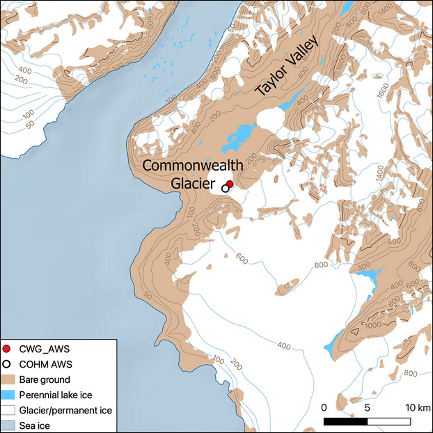
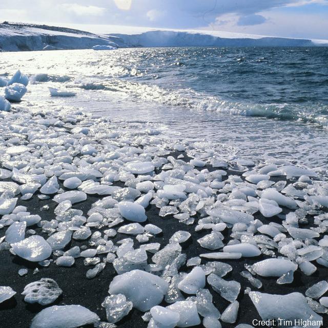
This metadata record represents the code and data used for the first application of WRF-Hydro/Glacier in the McMurdo Dry Valleys (Commonwealth Glacier), which as a fully distributed hydrological model has the capability to resolve the streams from the glaciers to the bare land that surround them. We applied a glacier and hydrology model in the McMurdo Dry Valleys (MDV) to model the start and duration of melt over a summer in this extreme polar desert. To do so, we found it necessary to prevent the drainage of melt into ice and optimize the albedo scheme. We show that simulating albedo (for the first time in the MDV) is critical to modelling the feedbacks of albedo, snowfall and melt in the region. This is a first step towards more complex spatial modelling of melt and streamflow. The Zenodo data includes output point data (*.csv) and namelist used in: Pletzer, T., Conway, J.P., Cullen, N.J., Eidhammer, T., & Katurji, M. (2024). The application and modification of WRF-Hydro/Glacier to a cold-based Antarctic glacier. *Hydrology and Earth System Sciences*, 28(3), 459-478. https://doi.org/10.5194/hess-28-459-2024 The modifications to the WRF-Hydro/Glacier model used in the paper can be found on GitHub: https://github.com/tpletzer/wrf_hydro_nwm_coldglacier GET DATA: https://doi.org/10.5281/zenodo.10565032

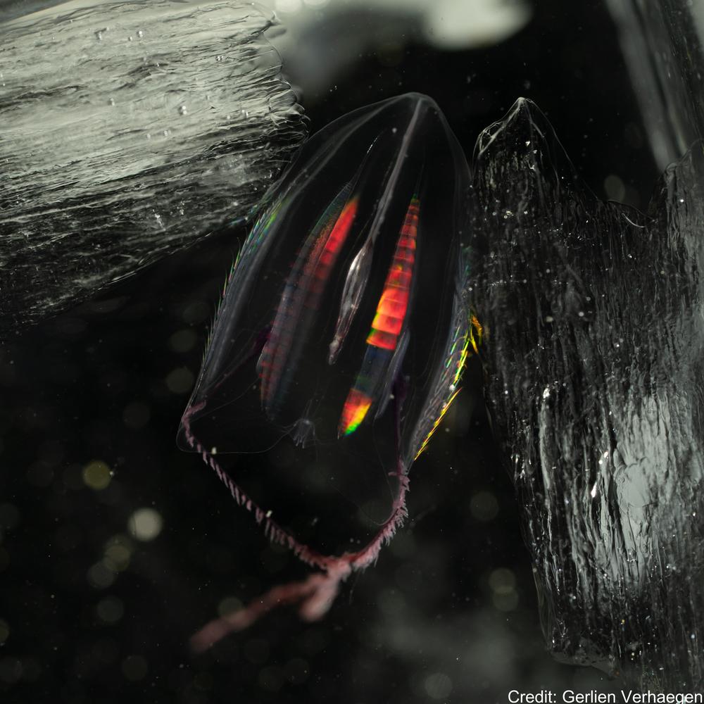
This Zenodo dataset contain the Common Objects in Context (COCO) files linked to the following publication: Each COCO zip folder contains an "annotations" folder including a json file and an "images" folder containing the annotated images. Verhaegen, G, Cimoli, E, & Lindsay, D (2021). Life beneath the ice: jellyfish and ctenophores from the Ross Sea, Antarctica, with an image-based training set for machine learning. Biodiversity Data Journal. https://doi.org/10.3897/BDJ.9.e69374 GET DATA: https://doi.org/10.5281/zenodo.5118012 GET DATA: http://ipt.pensoft.net/resource?r=life_beneath_the_ice-jellyfish_and_ctenophores_from_the_ross_sea_antarctica&v=1.3

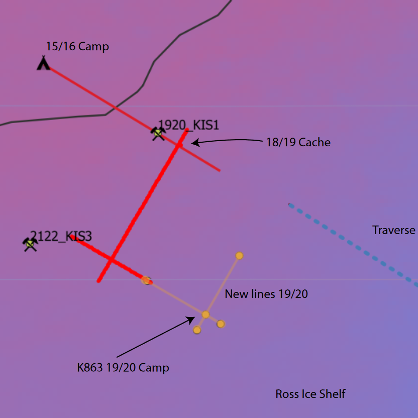
These data are described in detail by 'Melting and refreezing in an ice shelf basal channel at the grounding line of the Kamb Ice Stream 1/ HWD1. ApRES observations were made in December 2019 and repeated in December 2020 at the same locations. Data collection and processing followed the method described in Stewart et al. (2019). ApRES dataset.zip' contains raw ApRES data and processed results from a spatial survey of basal mass balance - detailed in Sections 2.2.4 and 3.2.2 of: Whiteford, A., Horgan, H. J., Leong, W. J., & Forbes, M. (2022). Melting and refreezing in an ice shelf basal channel at the grounding line of the Kamb Ice Stream, West Antarctica. Journal of Geophysical Research: Earth Surface, 127, e2021JF006532. https://doi.org/10.1029/2021JF006532 GET DATA: https://doi.org/10.5281/zenodo.5574647

This dataset contains 5 s average phase and amplitude data from VLF radio wave communication transmitters received on two subionospheric propagation paths. The first is the path from NPM (Hawaii, 21.4 kHz, 21.4⁰N, 158.2⁰E), recorded at the field-site for New Zealand's Scott Base, Arrival Heights, in Antarctica (77.8⁰S, 166.8⁰E). The propagation path is ~11 Mm long, oriented nearly north-south, with the mid-point at 28.9⁰S, 164.4⁰W. The second is from NAA (Culter, Maine, USA, 24.0 kHz, 44.7⁰N, 67.3⁰E), and recorded at Sodankylä Geophysical Observatory (Lapland, Finland, 67.4⁰N, 26.4⁰E). The propagation path is ~6 Mm. Both VLF recievers are UltraMSK software defined radio systems connected to magnetic field sensing loops. The data files are formatted as ASCII text files with columns of time (s), amplitude (dB) & phase (degrees) data. The MATLAB script plotUltraMSK.m can be used to plot the data files and an example data plot has been included in the dataset. Further details provided at: Belcher, S. R. G., Clilverd, M. A., Rodger, C. J., Cook, S., Thomson, N. R., Brundell, J. B., & Raita, T. (2021). Solar flare X-ray impacts on long subionospheric VLF paths. Space Weather, 19, e2021SW002820. https://doi.org/10.1029/2021SW002820 GET DATA: https://doi.org/10.5281/zenodo.4774464

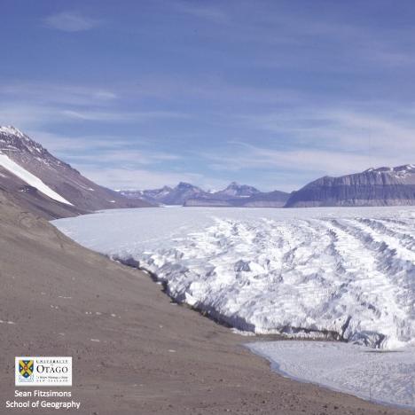
The structural glaciology and movement of the Taylor Glacier, was investigated over several seasons (98-01) by excavating a tunnel in the right side of the Taylor Glacier, 1.5km upstream of the terminus, to provide access to basal ice and the glacier substrate. Basal ice was sampled and analysed for concentration of base cations and chlorides present. Strain arrays and precision dial gauges were installed to monitor movement and deformation of the tunnel and ice velocity. In situ samples of clean and debris bearing glacier ice shear samples were taken from the basal ice to test in a laboratory. The tunnel was re-cut 1.3km upstream of the terminus in the 99-00 season as the other had closed in, with strain arrays and plumb lines installed and basal ice re-sampled. Ice cores were sampled for mechanical tests from the tunnel and the glacier surface. Ice cores were taken from the ice margin of Lake Bonny. Strain arrays and plumb lines were resurveyed and the deformation of the tunnel measured. This metadata record represents: - Data set from Taylor Glacier tunnel - Photographs of tunnel excavation - Video of tunnel excavation Further details are provided at: Fitzsimons, S., Samyn, D., & Lorrain, R (2024). Deformation, strength and tectonic evolution of basal ice in Taylor Glacier, Antarctica. Journal of Geophysical Research: Earth Surface, 129, e2023JF007456. https://doi.org/10.1029/2023JF007456 GET DATA: https://doi.org/10.5281/zenodo.8232003

GET DATA: https://doi.org/10.5281/zenodo.3940766 This archive provides the ice sheet model outputs produced as part of the publication "ISMIP6 Antarctica: a multi-model ensemble of the Antarctic ice sheet evolution over the 21st century", published in The Cryosphere, https://tc.copernicus.org/articles/14/3033/2020/ Contact: Helene Seroussi, Helene.seroussi@jpl.nasa.gov Further information on ISMIP6 and ISMIP6 Antarctica Projections can be found here: http://www.climate-cryosphere.org/activities/targeted/ismip6 http://www.climate-cryosphere.org/wiki/index.php?title=ISMIP6-Projections-Antarctica Users should cite the original publication when using all or part of the data. In order to document CMIP6’s scientific impact and enable ongoing support of CMIP, users are also obligated to acknowledge CMIP6, ISMIP6 and the participating modeling groups. About the dataset: - The results are based on model output computed from the ISMIP6 native grids that vary between models. - The results are calculated over the ice-covered area of Antarctica, corrected for map projection errors, ice sheet model specific densities taken into account. - Results for the experiments 'exp*' are provided both as raw results and calculated as differences to the control experiment (ctrl_proj_open or ctrl_proj_std depending on the experiment). The later files are named with "minus_ctrl_proj" to indicate that the control run is substracted. - Results for ctrl_proj_open, ctrl_proj_std, hist_open and hist_std are not corrected to remove the control run. ----------------> Directory structure: groupname1 modelname1 expid computed_iareafl_AIS_groupname1_modelname1_expid.nc computed_iareafl_minus_ctrl_proj_AIS_groupname1_modelname1_expid.nc computed_iareagr_AIS_groupname1_modelname1_expid.nc computed_iareagr_minus_ctrl_proj_AIS_groupname1_modelname1_expid.nc computed_icearea_AIS_groupname1_modelname1_expid.nc computed_icearea_minus_ctrl_proj_AIS_groupname1_modelname1_expid.nc computed_ivol_AIS_groupname1_modelname1_expid.nc computed_ivol_minus_ctrl_proj_AIS_groupname1_modelname1_expid.nc computed_ivaf_AIS_groupname1_modelname1_expid.nc computed_ivaf_minus_ctrl_proj_AIS_groupname1_modelname1_expid.nc computed_smb_AIS_groupname1_modelname1_expid.nc computed_smb_minus_ctrl_proj_AIS_groupname1_modelname1_expid.nc computed_smbgr_AIS_groupname1_modelname1_expid.nc computed_smbgr_minus_ctrl_proj_AIS_groupname1_modelname1_expid.nc computed_bmbfl_AIS_groupname1_modelname1_expid.nc computed_bmbfl_minus_ctrl_proj_AIS_groupname1_modelname1_expid.nc ... ----------> Description of variables: icearea - ice area [m^2] iareafl - floating ice area [m^2] iareagr - grounded ice area [m^2] ivol - ice volume [m^3] ivaf - ice volume above floatation [m^3] smb - spatially integrated surface mass balance [kg/s] smbgr - spatially integrated surface mass balance over grounded ice [kg/s] bmbfl - spatially integrated basal melt rate under floating ice (negative for melting ice) [kg/s] Variables per file: rhoi - model specific ice density [kg m-3] rhow - model specific ocean water density [kg m-3] time - time, in years [variable] - global variable integrated over the Antarctica ice sheet [variable]_region_1 - variable integrated over West Antarctica [variable]_region_2 - variable integrated over East Antarctica [variable]_region_3 - variable integrated over the Antarctic Peninsula [variable]_sector_X - variable integrated over the X sector of the Antarctic ice sheet (18 sectors, from 1 to 18) -------------------> Data usage notice: If you use any of these results, please acknowledge the work of the people involved in producing them. Acknowledgements should have language similar to the below. "We thank the Climate and Cryosphere (CliC) effort, which provided support for ISMIP6 through sponsoring of workshops, hosting the ISMIP6 website and wiki, and promoted ISMIP6. We acknowledge the World Climate Research Programme, which, through it's Working Group on Coupled Modelling, coordinated and promoted CMIP5 and CMIP6. We thank the climate modeling groups for producing and making available their model output, the Earth System Grid Federation (ESGF) for archiving the CMIP data and providing access, the University at Buffalo for ISMIP6 data distribution and upload, and the multiple funding agencies who support CMIP5 and CMIP6 and ESGF. We thank the ISMIP6 steering committee, the ISMIP6 model selection group and ISMIP6 dataset preparation group for their continuous engagement in defining ISMIP6." You should also refer to and cite the following papers: https://doi.org/10.5194/tc-14-3033-2020, 2020. https://doi.org/10.5194/tc-14-2331-2020, 2020.